Latency and Bandwidth
This is a practical example of how the characteristics of a parallel computer determine program optimization. It is based on a real-world physics endeavor. The parallel computers used cost hundreds of thousands of dollars and even small optimizations of 10-20% save thousands of dollars!
The Setup
The specifics of the problem have been simplified in order to illustrate the key ideas. The premise is as follows:
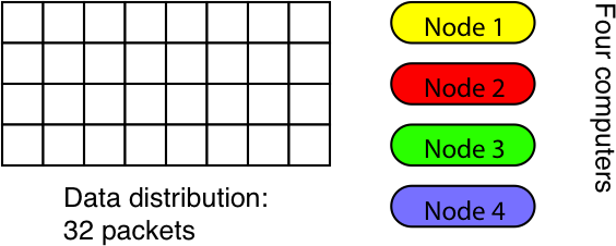
- Data is distributed over a plane. For the purpose of this discussion the distribution consists of data packets arranged on a 4x8 grid, i.e., there are 32 chunks of data that need to be handled.
- The computer has four nodes. Each node is working on 16 data packets, doing an identical series of operations on each.
- The computation involves talking to nearest-neighbors only, i.e., each data packet needs information from the one to its left, right, above and below. (We do not deal with a shared-memory architecture, i.e., the communication is a genuine non-trivial operation.)
- The data is arranged like a torus, i.e., the neighbors of data packets at the border are located across at the opposite border.
- The bottleneck is communication. Whereas the computations on each packet are simple, it is crucial to pass information to and from the neighbors as fast as possible.
This type of arrangement is quite common and is referred to as SIMD (single instruction, multiple data). It means that each node executes the same instructions (a “single instruction” at a time), but acts on different data each (“multiple data”).
Question: What is the optimal distribution of the data on the nodes?
It depends!
In the following I want to talk about different perspectives on this problem.
Latency vs Bandwidth
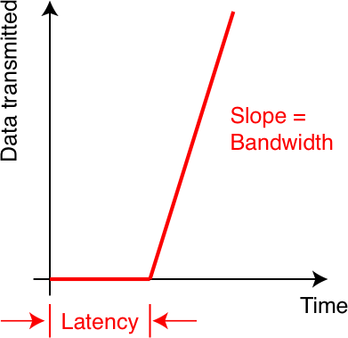
Let me talk about two characteristics of communication: latency and bandwidth. Latency refers to the time it takes to initiate a communication. Bandwidth describes how fast you can get information across. A real-life example of high latency may be a service call to your cell phone company: First, you need to find the number, next you have to dial it, then you wait in the loop for what seems like ages, subsequently you get passed along until you finally reach someone who can solve your problem. Bandwidth corresponds to the other part: how long you need to describe the problem once you reached the correct person to talk to.
Thus, how long a communication takes depends on two factors: the time to initiate it (the latency) plus the amount of information you need to transfer multiplied by the speed at which it can be transmitted (the bandwidth). Graphically, it looks like this:
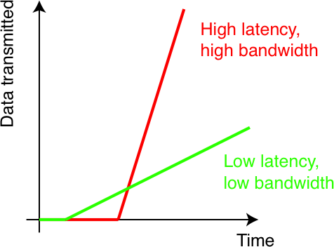
We need to know what the latency and the bandwidth of our machine. In general, this is machine dependent. It is usually not enough to just focus on the mathematical part of the problem. Of equal importance is the implementation system itself.
Implementation Systems
When actually doing the above computation there were several implementation systems with different features. The most prominent two we had at our disposal were:
- The Quadrics/APE
- The APE 100 was a SIMD parallel computer developed at the INFN in Italy. It had zero latency by design, thus the number of communications did not matter. Only the amount of data that is communicated matters. For this machine it pays to minimize the amount of data being transferred.
- Cluster computers
- For computer clusters build from off-the-shelf components the network may be fast but may have a non-negligible latency. In the above case it turned out that the latency was a significant factor and practically dominated the communication for the data sizes in question. Thus, it was imperative to minimize the number of communications even if it means to communicate more data.
What does this mean in practice? It means that the optimal distribution was different in each case. For the Quadrics/APE it was key to minimize the amount of data being communicated. For cluster computers it was crucial to keep the number of communications as low as possible.
The Solution
Computer Clusters
For the computer clusters the best solution was to distribute the data on the nodes as depicted here:
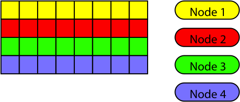
The colors refer to the node the data is located on. Since the data of a complete slice resides on each node there is no need to communicate the left/right boundaries and the only communication is above and below. Each node thus has two communication operations to perform, one to the node above and another one to the node below. The amount of data that needs to be transferred is sixteen packets.
Quadrics/APE
On the other hand for the Quadrics/APE machine the optimal distribution is different:
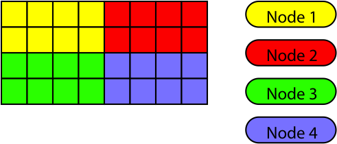
The total number of communication operations is now four since each node needs to talk to neighbors above and below PLUS left and right. On the other hand the amount of data chunks that is communicated is only twelve (four each to neighbors below and above and two each to the left and right).
A different way to formulate this finding is to say that the data volume per node is identical, but the “surfaces” are not. The data surface is larger on the cluster computer and smaller on the APE/Quadrics. In general, smaller surfaces minimize the amount of data that needs to be communicated. However, for the computer cluster a preferred shape served to minimize the total communication time, a finding that appears counter-intuitive at first.
Conclusion
It was possible and indeed beneficial to trade more data for fewer communications in one case and vice versa in the other. The real-world example actually was more complicated and involved hundreds of nodes in a three-dimensional grid and a tree-shaped network and more than one hundred thousand data packets arranged in a four-dimensional grid. But the key to optimization was the same as in this example: Find the data distribution that optimally fits the characteristics of the machine!
Since the machines actually cost hundreds of thousands of dollars such optimizations can literally be worth thousands of dollars!